Motivation
Recently I spent a considerable amount of time writing the postman_problems python library implementing solvers for the Chinese and Rural Postman Problems (CPP and RPP respectively). I wrote about my initial motivation for the project: finding the optimal route through a trail system in a state park here. Although I’ve still yet to run the 34 mile optimal trail route, I am pleased with the optimization procedure. However, I couldn’t help but feel that all those nights and weekends hobbying on this thing deserved a more satisfying visual than my static SVGs and hacky GIF. So to spice it up, I decided to solve the RPP on a graph derived from geodata and visualize on an interactive Leaflet map.
The Problem
In short, ride all 50 state named avenues in DC end-to-end following the shortest route possible.
There happens to be an annual 50 states ride sponsored by our regional bike association, WABA, that takes riders to each of the 50† state named avenues in DC. Each state’s avenue is touched, but not covered in full. This problem takes it a step further by instituting this requirement. Thus, it boils to the RPP where the required edges are state avenues (end-to-end) and the optional edges are every other road within DC city limits.
For those unfamiliar with DC street naming convention, that can (and should) be remedied with a read through the history behind the street system here. Seriously, it’s an interesting read. Basically there are 50 state named avenues in DC ranging from 0.3 miles (Indiana Avenue) to 10 miles (Massachusetts Avenue) comprising 115 miles in total.
The Solution
The data is grabbed from Open Street Maps (OSM). Most of the post is spent wrangling the OSM geodata into shape for the RPP algorithm using NetworkX graphs. The final route (and intermediate steps) are visualized using Leaflet maps through mplleaflet which enable interactivity using tiles from Mapbox and CartoDB among others.
Note to readers: the rendering of these maps can work the browser pretty hard; allow a couple extra seconds for loading.
The Approach
Most of the heavy lifting leverages functions from the graph.py module in the postman_problems_examples repo. The majority of pre-RPP processing employs heuristics that simplify the computation such that this code can run in a reasonable amount of time. The parameters employed here, which I believe get pretty darn close to the optimal solution, run in about 50 minutes. By tweaking a couple parameters, accuracy can be sacrificed for time to get run time down to ~5 minutes on a standard 4 core laptop.
Verbose technical details about the guts of each step are omitted from this post for readability. However the interested reader can find these in the docstrings in graph.py.
The table of contents below provides the best high-level summary of the approach. All code needed to reproduce this analysis is in the postman_problems_examples repo, including the jupyter notebook used to author this blog post and a conda environment.
† While there are 50 roadways, there are technically only 48 state named avenues: Ohio Drive and California Street are the stubborn exceptions.
Table of Contents
- 0: Get the data
- 1: Load OSM to NetworkX
- 2: Make Graph w State Avenues only
- 3. Remove Redundant State Avenues
- 4. Create Single Connected Component
- 5. Solve CPP
- 6. Solve RPP
import mplleaflet
import networkx as nx
import pandas as pd
import matplotlib.pyplot as plt
from collections import Counter

# can be found in https://github.com/brooksandrew/postman_problems_examples
from osm2nx import read_osm, haversine
from graph import (
    states_to_state_avenue_name, subset_graph_by_edge_name, keep_oneway_edges_only, create_connected_components,
    create_unkinked_connected_components, nodewise_distance_connected_components,
    calculate_component_overlap, calculate_redundant_components, create_deduped_state_road_graph,
    create_contracted_edge_graph, shortest_paths_between_components, find_minimum_weight_edges_to_connect_components,
    create_rpp_edgelist
    )

# can be found in https://github.com/brooksandrew/postman_problems
from postman_problems.tests.utils import create_mock_csv_from_dataframe
from postman_problems.solver import rpp, cpp
from postman_problems.stats import calculate_postman_solution_stats
0: Get the data
There are many ways to grab Open Street Map (OSM) data, since it’s, well, open. I grabbed the DC map from GeoFabrik here.
1: Load OSM to NetworkX
While some libraries like OSMnx provide an elegant interface to downloading, transforming and manipulating OSM data in NetworkX, I decided to start with the raw
data itself. I adopted an OSM-to-nx parser from a hodge podge of Gists (here and there) to read_osm.
read_osm creates a directed graph. However, for this analysis, we’ll use undirected graphs with the assumption that all roads are bidirectional on a bike one way or another.
%%time

# load OSM to a directed NX
g = read_osm('district-of-columbia-latest.osm')

# create an undirected graph
g_ud = g.to_undirected()
<class 'networkx.classes.digraph.DiGraph'>
CPU times: user 46.6 s, sys: 2.1 s, total: 48.7 s
Wall time: 50.2 s
This is a pretty big graph, about 275k edges. It takes about a minute to load on my machine (Macbook w 4 cores)
print(len(g.edges())) # number of edges275429
2: Make Graph w State Avenues only
Generate state avenue names
STATE_STREET_NAMES = [
    'Alabama','Alaska','Arizona','Arkansas','California','Colorado',
    'Connecticut','Delaware','Florida','Georgia','Hawaii','Idaho','Illinois',
    'Indiana','Iowa','Kansas','Kentucky','Louisiana','Maine','Maryland',
    'Massachusetts','Michigan','Minnesota','Mississippi','Missouri','Montana',
    'Nebraska','Nevada','New Hampshire','New Jersey','New Mexico','New York',
    'North Carolina','North Dakota','Ohio','Oklahoma','Oregon','Pennsylvania',
    'Rhode Island','South Carolina','South Dakota','Tennessee','Texas','Utah',
    'Vermont','Virginia','Washington','West Virginia','Wisconsin','Wyoming'
]
Most state avenues are written in the long form (ex. Connecticut Avenue Northwest). However, some, such as Florida Ave NW, are written in the short form. To be safe, we grab any permutation OSM could throw at us.
candidate_state_avenue_names = states_to_state_avenue_name(STATE_STREET_NAMES)

# two states break the "Avenue" pattern
candidate_state_avenue_names += ['California Street Northwest', 'Ohio Drive Southwest']

# preview
candidate_state_avenue_names[0:20]
['Alabama Ave Southeast',
'Alabama Ave Southwest',
'Alabama Ave Northeast',
'Alabama Ave Northwest',
'Alabama Ave SE',
'Alabama Ave SW',
'Alabama Ave NE',
'Alabama Ave NW',
'Alabama Avenue Southeast',
'Alabama Avenue Southwest',
'Alabama Avenue Northeast',
'Alabama Avenue Northwest',
'Alabama Avenue SE',
'Alabama Avenue SW',
'Alabama Avenue NE',
'Alabama Avenue NW',
'Alaska Ave Southeast',
'Alaska Ave Southwest',
'Alaska Ave Northeast',
'Alaska Ave Northwest']
Create graph w state avenues only
g_st = subset_graph_by_edge_name(g, candidate_state_avenue_names)

# Add state edge attribute from full streetname (with avenue/drive and quandrant)
for e in g_st.edges(data=True):
    e[2]['state'] = e[2]['name'].rsplit(' ', 2)[0]
This is a much smaller graph:
print(len(g_st.edges()))7148
But every state is represented:
edge_count_by_state = Counter([e[2]['state'] for e in g_st.edges(data=True)])

# number of unique states
print(len(edge_count_by_state))
50
Here they are by edge count:
edge_count_by_stateCounter({'Alabama': 348,
'Alaska': 36,
'Arizona': 89,
'Arkansas': 64,
'California': 24,
'Colorado': 59,
'Connecticut': 283,
'Delaware': 66,
'Florida': 253,
'Georgia': 185,
'Hawaii': 84,
'Idaho': 50,
'Illinois': 37,
'Indiana': 29,
'Iowa': 30,
'Kansas': 74,
'Kentucky': 47,
'Louisiana': 37,
'Maine': 199,
'Maryland': 233,
'Massachusetts': 581,
'Michigan': 225,
'Minnesota': 214,
'Mississippi': 102,
'Missouri': 66,
'Montana': 74,
'Nebraska': 183,
'Nevada': 122,
'New Hampshire': 259,
'New Jersey': 170,
'New Mexico': 66,
'New York': 333,
'North Carolina': 87,
'North Dakota': 16,
'Ohio': 391,
'Oklahoma': 48,
'Oregon': 170,
'Pennsylvania': 433,
'Rhode Island': 282,
'South Carolina': 60,
'South Dakota': 124,
'Tennessee': 40,
'Texas': 123,
'Utah': 66,
'Vermont': 154,
'Virginia': 134,
'Washington': 58,
'West Virginia': 56,
'Wisconsin': 257,
'Wyoming': 27})
2.1 Viz state avenues
As long as your NetworkX graph has lat and lon node attributes, mplleaflet can be used to pretty effortlessly plot your NetworkX graph on an interactive map.
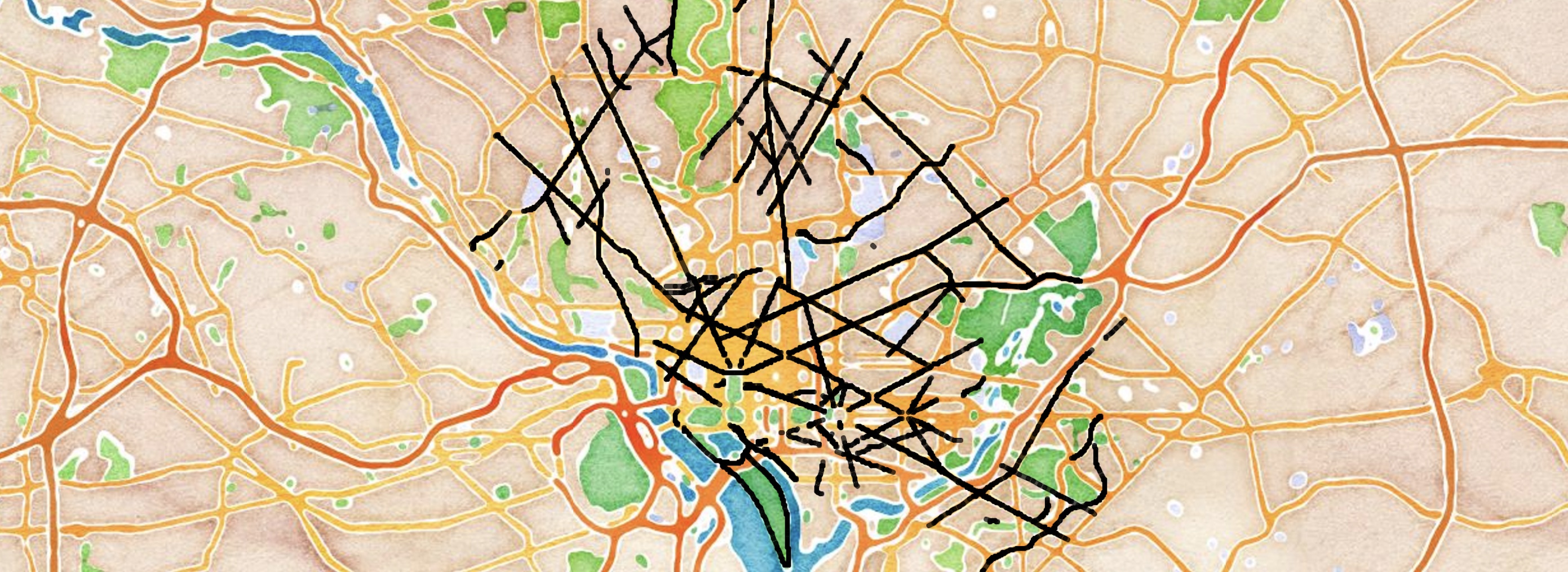
Here’s the map with all the state avenues…
fig, ax = plt.subplots(figsize=(1,8))

pos = {k: (g_st.node[k]['lon'], g_st.node[k]['lat']) for k in g_st.nodes()}
nx.draw_networkx_edges(g_st, pos, width=4.0, edge_color='black', alpha=0.7)

# save viz
mplleaflet.save_html(fig, 'state_avenues_all.html', tiles='cartodb_positron')
You can even customize with your favorite tiles. For example:
mplleaflet.display(fig=ax.figure, tiles='stamen_wc')

…But there’s a wrinkle. Zoom in on bigger avenues, like New York or Rhode Island, and you’ll notice that there are two parallel edges representing each direction as a separate one-way road. This usually occurs when there are several lanes of traffic in each direction, or physical dividers between directions. Example below:
This is great for OSM and point A to B routing problems, but for the Rural Postman problem it imposes the requirement that each main avenue be cycled twice. We’re not into that.
Example: Rhode Island Ave (parallel edges) vs Florida Ave (single edge)

3. Remove Redundant State Avenues
As it turns out, removing these parallel (redundant) edges is a nontrivial problem to solve. My approach is the following:
- Build graph with one-way state avenue edges only.
- For each state avenue, create list of connected components that represent sequences of OSM ways in the same direction (broken up by intersections and turns).
- Compute distance between each node in a component to every other node in the other candidate components.
- Identify redundant components as those with the majority of their nodes below some threshold distance away from another component.
- Build graph without redundant edges.
3.1 Create state avenue graph with one-way edges only
g_st1 = keep_oneway_edges_only(g_st)The one-way avenues are plotted in red below. A brief look indicates that 80-90% of the one-way avenues are parallel (redundant). A few, like Idaho Avenue NW and Ohio Drive SW, are single one-way roads with no accompanying parallel edge for us to remove.
NOTE: you’ll need to zoom in 3-4 levels to see the parallel edges.
fig, ax = plt.subplots(figsize=(1,6))

pos = {k: (g_st1.node[k]['lon'], g_st1.node[k]['lat']) for k in g_st1.nodes()}
nx.draw_networkx_edges(g_st1, pos, width=3.0, edge_color='red', alpha=0.7)

# save viz
mplleaflet.save_html(fig, 'oneway_state_avenues.html', tiles='cartodb_positron')
Create connected components with one-way state avenues
comps = create_connected_components(g_st1)There are 163 distinct components in the graph above.
len(comps)163
3.2 Split connected components
Remove kinked nodes
However, we need to break some of these components up into smaller ones. Many components, like the one below, have bends or a connected cycle that contain both the parallel edges, where we only want one. My approach is to identify the nodes with sharp angles and remove them. I don’t know what the proper name for these is (you can read about angular resolution), but we’ll call them “kinked nodes.”
This will split the connected component below into two, allowing us to determine that one of them is redundant.

I borrow this code from jeromer to calculate the compass bearing (0 to 360) of each edge. Wherever the the bearing difference between two adjacent edges is greater than
bearing_thresh, we call the node shared by both edges a “kinked node.” A relative low bearing_thresh of 60 appeared to work best after some experimentation.
# create list of comps (graphs) without kinked nodes
comps_unkinked = create_unkinked_connected_components(comps=comps, bearing_thresh=60)

# comps in dict form for easy lookup
comps_dict = {comp.graph['id']:comp for comp in comps_unkinked}
After removing these “kinked nodes,” our list of components grows from 163 to 246:
len(comps_unkinked)246
Viz components without kinked nodes
Example: Here’s the Massachusetts Ave example from above after we remove kinked nodes:

Full map: Zoom in on the map below and you’ll see that we split up most of the obvious components that should be. There are a few corner cases that we miss, but I’d estimate we programmatically split about 95% of the components correctly.
fig, ax = plt.subplots(figsize=(1,6))

for comp in comps_unkinked:
    pos = {k: (comp.node[k]['lon'], comp.node[k]['lat']) for k in comp.nodes()}
    nx.draw_networkx_edges(comp, pos, width=3.0, edge_color='orange', alpha=0.7)

mplleaflet.save_html(fig, 'oneway_state_avenues_without_kinked_nodes.html', tiles='cartodb_positron')
3.3 & 3.4 Match connected components
Now that we’ve crafted the right components, we calculate how close (parallel) each component is to one another.
This is a relatively coarse approach, but performs surprisingly well:
1. Find closest nodes from candidate components to each node in each component (pseudo code below):
  For each node N in component C:
    For each C_cand in components with same street avenue as C:
      Calculate closest node in C_cand to N.
2. Calculate overlap between components. Using the distances calculated in 1., we say that a node from component C is matched to a component C_cand if the distance is less than
thresh_distance specified in calculate_component_overlap. 75 meters seemed to work pretty well. Essentially we’re saying these nodes are close enough to be considered interchangeable.
3. Use the node-wise matching calculated in 2. to calculate which components are redundant. If thresh_pct of nodes in component C are close enough (within thresh_distance) to nodes in
component C_cand, we call C redundant and discard it.
# caclulate nodewise distances between each node in comp with closest node in each candidate
comp_matches = nodewise_distance_connected_components(comps_unkinked)

# calculate overlap between components
comp_overlap = calculate_component_overlap(comp_matches, thresh_distance=75)

# identify redundant and non-redundant components
remove_comp_ids, keep_comp_ids = calculate_redundant_components(comp_overlap, thresh_pct=0.75)
Viz redundant component solution
The map below visualizes the solution to the redundant parallel edges problem. There are some misses, but overall this simple approach works surprisingly well:
- red: redundant one-way edges to remove
- black: one-way edges to keep
- blue: all state avenues
fig, ax = plt.subplots(figsize=(1,8))

# plot redundant one-way edges
for i, road in enumerate(remove_comp_ids):
    for comp_id in remove_comp_ids[road]:
        comp = comps_dict[comp_id]
        posc = {k: (comp.node[k]['lon'], comp.node[k]['lat']) for k in comp.nodes()}
        nx.draw_networkx_edges(comp, posc, width=7.0, edge_color='red')

# plot keeper one-way edges
for i, road in enumerate(keep_comp_ids):
    for comp_id in keep_comp_ids[road]:
        comp = comps_dict[comp_id]
        posc = {k: (comp.node[k]['lon'], comp.node[k]['lat']) for k in comp.nodes()}
        nx.draw_networkx_edges(comp, posc, width=3.0, edge_color='black')

# plot all state avenues
pos_st = {k: (g_st.node[k]['lon'], g_st.node[k]['lat']) for k in g_st.nodes()}
nx.draw_networkx_edges(g_st, pos_st, width=1.0, edge_color='blue', alpha=0.7)

mplleaflet.save_html(fig, 'redundant_edges.html', tiles='cartodb_positron')
3.5 Build graph without redundant edges
This is the essentially the graph with just black and blue edges from the map above.
# create a single graph with deduped state roads
g_st_nd = create_deduped_state_road_graph(g_st, comps_dict, remove_comp_ids)
After deduping the redundant edges, our connected component count drops from 246 to 96.
len(list(nx.connected_components(g_st_nd)))96
4. Create Single Connected Component
The strategy I employ for solving the Rural Postman Problem (RPP) in postman_problems is simple in that it reuses the machinery from the Chinese Postman Problem (CPP) solver here. However, it makes the strong assumption that the graph’s required edges form a single connected component. This is obviously not true for our state avenue graph as-is, but it’s not too off. Although there are 96 components, there are only a couple more than a few hundred meters to the next closest component.
So we hack it a bit by adding required edges to the graph to make it a single connected component. The tricky part is choosing the edges that add as little distance as possible. This was the first computationally intensive step that required some clever tricks and approximations to ensure execution in a reasonable amount of time.
My approach:
-
Build graph with contracted edges only.
-
Calculate haversine distance between each possible pair of components.
-
Find minimum distance connectors: iterate through the data structure created in 2. to calculate shortest paths for top candidates based on haversine distance and add shortest connectors to graph. More details below.
-
Build single component graph.
4.1 Contract edges
Nodes with degree 2 are collapsed into an edge stretching from a dead-end node (degree 1) or intersection (degree >= 3) to another. This achieves two things:
- Limits the number of distance calculations.
- Ensures that components are connected at logical points (dead ends and intersections) rather than arbitrary parts of a roadway. This will make for a more continuous route.
# Create graph with contracted edges only
g_st_contracted = create_contracted_edge_graph(graph=g_st_nd,
                                               edge_weight='length')
This significantly reduces the nodes needed for distances computations by a factor of > 15.
print('Number of nodes in contracted graph: {}'.format(len(g_st_contracted.nodes())))
print('Number of nodes in original graph: {}'.format(len(g_st_nd.nodes())))
Number of nodes in contracted graph: 347
Number of nodes in original graph: 5962
4.2 Calculate haversine distance between components
The 345 nodes from the contracted edge graph translate to >100,000 possible node pairings. That means >100,000 distance calculations. While applying a shortest path algorithm over the graph would certainly be more exact, it is painfully slow compared to simple haversine distance. This is mainly due to the high number of nodes and edges in the DC OSM map (over 250k edges).
On my laptop I averaged about 4 shortest path calculations per second. Not too bad for a handful, but 115k would take about 7 hours. Haversine distance, by comparison, churns through 115k in a couple seconds.
# create dataframe with shortest paths (haversine distance) between each component
dfsp = shortest_paths_between_components(g_st_contracted)dfsp.shape[0] # number of rows (node pairs)116526
4.3 Find minimum distance connectors
This gets a bit tricky. Basically we iterate through the top (closest) candidate pairs of components and connect them iteration-by-iteration with the shortest path edge. We use pre-calculated haversine distance to get in the right ballpark, then refine with true shortest path for the closest 20 candidates. This helps us avoid the scenario where we naively connect two nodes that are geographically close as the crow flies (haversine), but far away via available roads. Two nodes separated by highways or train tracks, for example.
# min weight edges that create a single connected component
connector_edges = find_minimum_weight_edges_to_connect_components(dfsp=dfsp,
                                                                  graph=g_ud,
                                                                  edge_weight='length',
                                                                  top=20)
We had 96 components to connect, so it makes sense that we have 95 connectors.
len(connector_edges)95
4.4 Build single component graph
# adding connector edges to create one single connected component
for e in connector_edges:
    g_st_contracted.add_edge(e[0], e[1], distance=e[2]['distance'], path=e[2]['path'], required=1, connector=True)
We add about 12 miles with the 95 additional required edges. That’s not too bad: an average distance of 0.13 miles per each edge added.
print(sum([e[2]['distance'] for e in g_st_contracted.edges(data=True) if e[2].get('connector')])/1609.34)12.341087779659958
So that leaves us with a single component of 125 miles of required edges to optimize a route through. That means the distance of deduped state avenues alone, without connectors (~112 miles) is just a couple miles away from what Wikipedia reports (115 miles).
print(sum([e[2]['distance'] for e in g_st_contracted.edges(data=True)])/1609.34)125.06645388481837
Make graph with granular edges (filling in those that were contracted) connecting components:
g1comp = g_st_contracted.copy()
for e in g_st_contracted.edges(data=True):
    if 'path' in e[2]:
        granular_type = 'connector' if 'connector' in e[2] else 'state'

        # add granular connector edges to graph
        for pair in list(zip(e[2]['path'][:-1], e[2]['path'][1:])):
            g1comp.add_edge(pair[0], pair[1], granular='True', granular_type=granular_type)

        # add granular connector nodes to graph
        for n in e[2]['path']:
            g1comp.add_node(n, lat=g.node[n]['lat'], lon=g.node[n]['lon'])
4.5 Viz single connected component
Black edges represent the deduped state avenues. Red edges represent the 12 miles of connectors that create the single connected component.
fig, ax = plt.subplots(figsize=(1,6))

g1comp_conn = g1comp.copy()
g1comp_st = g1comp.copy()

for e in g1comp.edges(data=True):
    if ('granular_type' not in e[2]) or (e[2]['granular_type'] != 'connector'):
        g1comp_conn.remove_edge(e[0], e[1])

for e in g1comp.edges(data=True):
    if ('granular_type' not in e[2]) or (e[2]['granular_type'] != 'state'):
        g1comp_st.remove_edge(e[0], e[1])

pos = {k: (g1comp_conn.node[k]['lon'], g1comp_conn.node[k]['lat']) for k in g1comp_conn.nodes()}
nx.draw_networkx_edges(g1comp_conn, pos, width=5.0, edge_color='red')

pos_st = {k: (g1comp_st.node[k]['lon'], g1comp_st.node[k]['lat']) for k in g1comp_st.nodes()}
nx.draw_networkx_edges(g1comp_st, pos_st, width=3.0, edge_color='black')

# save viz
mplleaflet.save_html(fig, 'single_connected_comp.html', tiles='cartodb_positron')
5. Solve CPP
I don’t expect the Chinese Postman solution to be optimal since it only utilizes the required edges. However, I do expect it to execute quickly and serve as a benchmark for the Rural Postman solution. In the age of “deep learning,” I agree with Smerity, baselines need more love.
5.1 Create CPP edgelist
The cpp solver I wrote operates off an edgelist (text file). This feels a bit clunky here, but it works.
# create list with edge attributes and "from" & "to" nodes
tmp = []
for e in g_st_contracted.edges(data=True):
    tmpi = e[2].copy()  # so we don't mess w original graph
    tmpi['start_node'] = e[0]
    tmpi['end_node'] = e[1]
    tmp.append(tmpi)

# create dataframe w node1 and node2 in order
eldf = pd.DataFrame(tmp)
eldf = eldf[['start_node', 'end_node'] + list(set(eldf.columns)-{'start_node', 'end_node'})]
The first two columns are interpeted as the from and to nodes; everything else as edge attributes.
eldf.head(3)| start_node | end_node | comp | name | connector | path | distance | required | |
|---|---|---|---|---|---|---|---|---|
| 0 | 3788079770 | 649840206 | 0.0 | Texas Avenue Southeast | NaN | [649840206, 649840209, 649840220, 30100500, 64... | 1244.893849 | 1 |
| 1 | 3788079770 | 49744479 | NaN | NaN | True | [3788079770, 49751669, 4630443674, 49751671, 4... | 674.458290 | 1 |
| 2 | 49765126 | 49765287 | 1.0 | Georgia Avenue Northwest | NaN | [49765126, 49765129, 49765130, 49765131, 49765... | 559.251509 | 1 |
5.2 CPP solver
Starting point
I fix the starting node for the solution to OSM node 49765113 which corresponds to (38.917002, -77.0364987): the intersection of New Hampshire Avenue NW, 16th St NW and U St NW… and also
the close to my house:

Solve
# create mockfilename
elfn = create_mock_csv_from_dataframe(eldf)

# solve
START_NODE = '49765113'  # New Hampshire Ave NW & U St NW.
circuit_cpp, gcpp = cpp(elfn, start_node=START_NODE)
5.3: CPP results
The CPP solution covers roughly 390,000 meters, about 242 miles. The optimal CPP route doubles the required distance, doublebacking every edge on average… definitely not ideal.
# circuit stats
calculate_postman_solution_stats(circuit_cpp)
OrderedDict([('distance_walked', 391523.723281576),
('distance_doublebacked', 190249.27638658223),
('distance_walked_once', 201274.44689499377),
('distance_walked_optional', 0),
('distance_walked_required', 391523.723281576),
('edges_walked', 688),
('edges_doublebacked', 337),
('edges_walked_once', 351),
('edges_walked_optional', 0),
('edges_walked_required', 688)])
6. Solve RPP
The RPP should improve the CPP solution as it considers optional edges that can drastically limit the amount of doublebacking.
We could add every possible edge that connects the required nodes, but it turns out that computation blows up quickly, and I’m not that patient. The get_shortest_paths_distances is the bottleneck
applying dijkstra path length on all possible combinations. There are ~14k pairs to calculate shortest path for (4 per second) which would take almost one hour.
However, we can use some heuristics to speed this up dramatically without sacrificing too much.
6.1 Create RPP edgelist
Ideally optional edges will be relatively short, since they are, well, optional. It is unlikely that the RPP algorithm will find that leveraging an optional edge that stretches from one corner of the
graph to another will be efficient. Thus we constrain the set of optional edges presented to the RPP solver to include only those less than max_distance.
I experimented with several thresholds. 3200 meters certainly took longer (~40 minutes), but yielded the best route results. I tried 4000m which ran for about 4 hours and returned a route with the same distance (160 miles) as the 3200m threshold.
%%time
dfrpp = create_rpp_edgelist(g_st_contracted=g_st_contracted,
                            graph_full=g_ud,
                            edge_weight='length',
                            max_distance=3200)
CPU times: user 34min 38s, sys: 20.5 s, total: 34min 59s
Wall time: 36min 3s
Check how many optional edges are considered (0=optional, 1=required):
Counter(dfrpp['required'])Counter({0: 16021, 1: 351})
6.2 RPP solver
Apply the RPP solver to the processed dataset.
%%time

# create mockfilename
elfn = create_mock_csv_from_dataframe(dfrpp)

# solve
circuit_rpp, grpp = rpp(elfn, start_node=START_NODE)
CPU times: user 7min 25s, sys: 1.68 s, total: 7min 27s
Wall time: 7min 31s
6.3 RPP results
As expected, the RPP route is considerably shorter than the CPP solution. The ~242 mile CPP route is cut significantly to ~160 with the RPP approach.
~26,000m (~161 miles) in total with ~59,000m (37 miles) of doublebacking. Not bad… but probably a 2-day ride.
# RPP route distance (miles)
print(sum([e[3]['distance'] for e in circuit_rpp])/1609.34)
161.58546891004886
# hack to convert 'path' from str back to list.  Caused by `create_mock_csv_from_dataframe`
for e in circuit_rpp:
    if type(e[3]['path']) == str:
exec('e[3]["path"]=' + e[3]["path"])calculate_postman_solution_stats(circuit_rpp)OrderedDict([('distance_walked', 260045.958535698),
('distance_doublebacked', 58771.511640704295),
('distance_walked_once', 201274.4468949937),
('distance_walked_optional', 51891.485571184385),
('distance_walked_required', 208154.47296451364),
('edges_walked', 447),
('edges_doublebacked', 96),
('edges_walked_once', 351),
('edges_walked_optional', 57),
('edges_walked_required', 390)])
As seen below, filling the contracted edges back in with the granular nodes adds considerably to the edge count.
print('Number of edges in RPP circuit (with contracted edges): {}'.format(len(circuit_rpp)))
print('Number of edges in RPP circuit (with granular edges): {}'.format(rppdf.shape[0]))
Number of edges in RPP circuit (with contracted edges): 447
Number of edges in RPP circuit (with granular edges): 9081
6.4 Viz RPP graph
Create RPP granular graph
Add the granular edges (that we contracted for computation) back to the graph.
# calc shortest path between optional nodes and add to g1comp graph
for e in [e for e in circuit_rpp if e[3]['required']==0] :

    # add granular optional edges to g1comp
    path = e[3]['path']
    for pair in list(zip(path[:-1], path[1:])):
        if g1comp.has_edge(pair[0], pair[1]):
            continue
        g1comp.add_edge(pair[0], pair[1], granular='True', granular_type='optional')

    # add granular nodes from optional edge paths to g1comp
    for n in path:
        g1comp.add_node(n, lat=g.node[n]['lat'], lon=g.node[n]['lon'])
Visualize RPP solution by edge type
- black: required state avenue edges
- red: required non-state avenue edges added to form single component
- blue: optional non-state avenue roads
fig, ax = plt.subplots(figsize=(1,12))

g1comp_conn = g1comp.copy()
g1comp_st = g1comp.copy()
g1comp_opt = g1comp.copy()

for e in g1comp.edges(data=True):
    if e[2].get('granular_type') != 'connector':
        g1comp_conn.remove_edge(e[0], e[1])

for e in g1comp.edges(data=True):
    #if e[2].get('name') not in candidate_state_avenue_names:
    if e[2].get('granular_type') != 'state':
        g1comp_st.remove_edge(e[0], e[1])

for e in g1comp.edges(data=True):
    if e[2].get('granular_type') != 'optional':
        g1comp_opt.remove_edge(e[0], e[1])


pos = {k: (g1comp_conn.node[k]['lon'], g1comp_conn.node[k]['lat']) for k in g1comp_conn.nodes()}
nx.draw_networkx_edges(g1comp_conn, pos, width=6.0, edge_color='red')

pos_st = {k: (g1comp_st.node[k]['lon'], g1comp_st.node[k]['lat']) for k in g1comp_st.nodes()}
nx.draw_networkx_edges(g1comp_st, pos_st, width=4.0, edge_color='black')

pos_opt = {k: (g1comp_opt.node[k]['lon'], g1comp_opt.node[k]['lat']) for k in g1comp_opt.nodes()}
nx.draw_networkx_edges(g1comp_opt, pos_opt, width=2.0, edge_color='blue')

# save vbiz
mplleaflet.save_html(fig, 'rpp_solution_edge_type.html', tiles='cartodb_positron')
Visualize RPP solution by edge walk count
Edge walks per color:
black: 1
magenta: 2
orange: 3
Edges walked more than once are also widened.
This solution feels pretty reasonable with surprisingly little doublebacking. After staring at this for several minutes, I could think of roads I’d prefer not to cycle on, but no obvious shorter paths.
## Create graph directly from rpp_circuit and original graph w lat/lon (g_ud)
color_seq = [None, 'black', 'magenta', 'orange', 'yellow']
grppviz = nx.Graph()
edges_cnt = Counter([tuple(sorted([e[0], e[1]])) for e in circuit_rpp])

for e in circuit_rpp:
    for n1, n2 in zip(e[3]['path'][:-1], e[3]['path'][1:]):
        if grppviz.has_edge(n1, n2):
            grppviz[n1][n2]['linewidth'] += 2
            grppviz[n1][n2]['cnt'] += 1
        else:
            grppviz.add_edge(n1, n2, linewidth=2.5)
            grppviz[n1][n2]['color_st'] = 'black' if g_st.has_edge(n1, n2) else 'red'
            grppviz[n1][n2]['cnt'] = 1
            grppviz.add_node(n1, lat=g_ud.node[n1]['lat'], lon=g_ud.node[n1]['lon'])
            grppviz.add_node(n2, lat=g_ud.node[n2]['lat'], lon=g_ud.node[n2]['lon'])

for e in grppviz.edges(data=True):
e[2]['color_cnt'] = color_seq[e[2]['cnt']]fig, ax = plt.subplots(figsize=(1,12))
pos = {k: (grppviz.node[k]['lon'], grppviz.node[k]['lat']) for k in grppviz.nodes()}
e_width = [e[2]['linewidth'] for e in grppviz.edges(data=True)]
e_color = [e[2]['color_cnt'] for e in grppviz.edges(data=True)]
nx.draw_networkx_edges(grppviz, pos, width=e_width, edge_color=e_color, alpha=0.7)
# save viz
mplleaflet.save_html(fig, 'rpp_solution_edge_cnt.html', tiles='cartodb_positron')6.5 Serialize RPP solution
CSV
Remember we contracted the edges in 4.1 for more efficient computation. However, when we visualize the solution, the more granular edges within the larger contracted ones are filled back in, so we can see the exact route to ride with all the bends and squiggles.
# fill in RPP solution edgelist with granular nodes
rpplist = []
for ee in circuit_rpp:
    path = list(zip(ee[3]['path'][:-1], ee[3]['path'][1:]))
    for e in path:
        rpplist.append({
            'start_node': e[0],
            'end_node': e[1],
            'start_lat': g_ud.node[e[0]]['lat'],
            'start_lon': g_ud.node[e[0]]['lon'],
            'end_lat': g_ud.node[e[1]]['lat'],
            'end_lon': g_ud.node[e[1]]['lon'],
            'street_name': g_ud[e[0]][e[1]].get('name')
        })

# write solution to disk
rppdf = pd.DataFrame(rpplist)
rppdf.to_csv('rpp_solution.csv', index=False)
Geojson
Similarly, we create a geojson object of the RPP solution using the time attribute to keep track of the route order. This data structure can be used for fancy js/d3 visualizations. Coming soon,
hopefully.
geojson = {'features':[], 'type': 'FeatureCollection'}
time = 0
path = list(reversed(circuit_rpp[0][3]['path']))

for e in circuit_rpp:
    if e[3]['path'][0] != path[-1]:
        path = list(reversed(e[3]['path']))
    else:
        path = e[3]['path']

    for n in path:
        time += 1
        doc = {'type': 'Feature',
              'properties': {
                  'latitude': g.node[n]['lat'],
                  'longitude': g.node[n]['lon'],
                  'time': time,
                  'id': e[3].get('id')
              },
              'geometry':{
                  'type': 'Point',
                  'coordinates': [g.node[n]['lon'], g.node[n]['lat']]
              }
          }
        geojson['features'].append(doc)
with open('circuit_rpp.geojson','w') as f:
json.dump(geojson, f)