This problem originated from a blog post I wrote for DataCamp on graph optimization here. The algorithm I sketched out there for solving the Chinese Problem on the Sleeping Giant state park trail network has since been formalized into the postman_problems python library. I’ve also added the Rural Postman solver that is implemented here.
So the three main enhancements in this post from the original DataCamp article and my second iteration published here updating to networkx 2.0 are:
- OpenStreetMap for graph data and visualization.
- Implementing the Rural Postman algorithm to consider optional edges.
- Leveraging the postman_problems library.
This code, notebook and data for this post can be found in the postman_problems_examples repo.
The motivation and background around this problem is written up more thoroughly in the previous posts and postman_problems.
RPP Solution Route Animation
Here’s the full route animation. More details here. Kudos to my sister @laurabrooks for coding this up!
Table of Contents
- Create Graph from OSM
- Viz Sleeping Giant Trails
- Connect Edges
- Viz Connected Component
- Viz Trail Color
- Contract Edges
- Solve CPP
- Solve RPP
- Viz RPP Solution
- Create geojson solution
import mplleaflet
import networkx as nx
import pandas as pd
import matplotlib.pyplot as plt
from collections import Counter

# can be found in https://github.com/brooksandrew/postman_problems_examples
from osm2nx import read_osm, haversine
from graph import contract_edges, create_rpp_edgelist

from postman_problems.tests.utils import create_mock_csv_from_dataframe
from postman_problems.solver import rpp, cpp
from postman_problems.stats import calculate_postman_solution_stats
Create Graph from OSM
# load OSM to a directed NX
g_d = read_osm('sleepinggiant.osm')

# create an undirected graph
g = g_d.to_undirected()
<class 'networkx.classes.digraph.DiGraph'>
Adding edges that don’t exist on OSM, but should
g.add_edge('2318082790', '2318082832', id='white_horseshoe_fix_1')Adding distance to OSM graph
Using the haversine formula to calculate distance between each edge.
for e in g.edges(data=True):
    e[2]['distance'] = haversine(g.node[e[0]]['lon'],
                                 g.node[e[0]]['lat'],
                                 g.node[e[1]]['lon'],
                                 g.node[e[1]]['lat'])
Create graph of required trails only
A simple heuristic with a couple tweaks is all we need to create the graph with required edges:
- Keep any edge with ‘Trail’ in the name attribute.
- Manually remove the handful of trails that are not part of the required Giant Master route.

g_t = g.copy()

for e in g.edges(data=True):

    # remove non trails
    name = e[2]['name'] if 'name' in e[2] else ''
    if ('Trail' not in name.split()) or (name is None):
        g_t.remove_edge(e[0], e[1])

    # remove non Sleeping Giant trails
    elif name in [
        'Farmington Canal Linear Trail',
        'Farmington Canal Heritage Trail',
        'Montowese Trail',
        '(white blazes)']:
        g_t.remove_edge(e[0], e[1])

# cleaning up nodes left without edges
for n in nx.isolates(g_t.copy()):
    g_t.remove_node(n)
Viz Sleeping Giant Trails
All trails required for the Giant Master:
fig, ax = plt.subplots(figsize=(1,8))

pos = {k: (g_t.node[k]['lon'], g_t.node[k]['lat']) for k in g_t.nodes()}
nx.draw_networkx_edges(g_t, pos, width=2.5, edge_color='black', alpha=0.7)

mplleaflet.save_html(fig, 'maps/sleepinggiant_trails_only.html')
Connect Edges
In order to run the RPP algorithm from postman_problems, the required edges of the graph must form a single connected component. We’re almost there with the Sleeping Giant trail map as-is, so we’ll just connect a few components manually.
Here’s an example of a few floating components (southwest corner of park):

OpenStreetMap makes finding these edge (way) IDs simple. Once grabbing the ? cursor, you can click on any edge to retrieve IDs and attributes.

Define OSM edges to add and remove from graph
edge_ids_to_add = [
    '223082783',
    '223077827',
    '40636272',
    '223082785',
    '222868698',
    '223083721',
    '222947116',
    '222711152',
    '222711155',
    '222860964',
    '223083718',
    '222867540',
    'white_horseshoe_fix_1'
]

edge_ids_to_remove = [
    '17220599'
]
Add attributes for supplementary edges
for e in g.edges(data=True):
    way_id = e[2].get('id').split('-')[0]
    if way_id in edge_ids_to_add:
        g_t.add_edge(e[0], e[1], **e[2])
        g_t.add_node(e[0], lat=g.node[e[0]]['lat'], lon=g.node[e[0]]['lon'])
        g_t.add_node(e[1], lat=g.node[e[1]]['lat'], lon=g.node[e[1]]['lon'])
    if way_id in edge_ids_to_remove:
        if g_t.has_edge(e[0], e[1]):
            g_t.remove_edge(e[0], e[1])

for n in nx.isolates(g_t.copy()):
    g_t.remove_node(n)
Ensuring that we’re left with one single connected component:
len(list(nx.connected_components(g_t)))1
Viz Connected Component
The map below visualizes the required edges and nodes of interest (intersections and dead-ends where degree != 2):
fig, ax = plt.subplots(figsize=(1,12))

# edges
pos = {k: (g_t.node[k].get('lon'), g_t.node[k].get('lat')) for k in g_t.nodes()}
nx.draw_networkx_edges(g_t, pos, width=3.0, edge_color='black', alpha=0.6)

# nodes (intersections and dead-ends)
pos_x = {k: (g_t.node[k]['lon'], g_t.node[k]['lat']) for k in g_t.nodes() if (g_t.degree(k)==1) | (g_t.degree(k)>2)}
nx.draw_networkx_nodes(g_t, pos_x, nodelist=pos_x.keys(), node_size=35.0, node_color='red', alpha=0.9)

mplleaflet.save_html(fig, 'maps/trails_only_intersections.html')
Viz Trail Color
Because we can and it’s pretty.
name2color = {
    'Green Trail': 'green',
    'Quinnipiac Trail': 'blue',
    'Tower Trail': 'black',
    'Yellow Trail': 'yellow',
    'Red Square Trail': 'red',
    'White/Blue Trail Link': 'lightblue',
    'Orange Trail': 'orange',
    'Mount Carmel Avenue': 'black',
    'Violet Trail': 'violet',
    'blue Trail': 'blue',
    'Red Triangle Trail': 'red',
    'Blue Trail': 'blue',
    'Blue/Violet Trail Link': 'purple',
    'Red Circle Trail': 'red',
    'White Trail': 'gray',
    'Red Diamond Trail': 'red',
    'Yellow/Green Trail Link': 'yellowgreen',
    'Nature Trail': 'forestgreen',
    'Red Hexagon Trail': 'red',
    None: 'black'
}fig, ax = plt.subplots(figsize=(1,10))
pos = {k: (g_t.node[k]['lon'], g_t.node[k]['lat']) for k in g_t.nodes()}
e_color = [name2color[e[2].get('name')] for e in g_t.edges(data=True)]
nx.draw_networkx_edges(g_t, pos, width=3.0, edge_color=e_color, alpha=0.5)
nx.draw_networkx_nodes(g_t, pos_x, nodelist=pos_x.keys(), node_size=30.0, node_color='black', alpha=0.9)
mplleaflet.save_html(fig, 'maps/trails_only_color.html', tiles='cartodb_positron')Check distance
This is strikingly close (within 0.25 miles) to what I calculated manually with some guess work from the SG trail map on the first pass at this problem here, before leveraging OSM.
print('{:0.2f} miles of required trail.'.format(sum([e[2]['distance']/1609.34 for e in g_t.edges(data=True)])))25.56 miles of required trail.
Contract Edges
We could run the RPP algorithm on the graph as-is with >5000 edges. However, we can simplify computation by contracting edges into logical trail segments first. More details on the intuition and methodology in the 50 states post.
print('Number of edges in trail graph: {}'.format(len(g_t.edges())))Number of edges in trail graph: 5141
# intialize contracted graph
g_tc = nx.MultiGraph()

# add contracted edges to graph
for ce in contract_edges(g_t, 'distance'):
    start_node, end_node, distance, path = ce

    contracted_edge = {
                'start_node': start_node,
                'end_node': end_node,
                'distance': distance,
                'name': g[path[0]][path[1]].get('name'),
                'required': 1,
                'path': path
            }

    g_tc.add_edge(start_node, end_node, **contracted_edge)
    g_tc.node[start_node]['lat'] = g.node[start_node]['lat']
    g_tc.node[start_node]['lon'] = g.node[start_node]['lon']
    g_tc.node[end_node]['lat'] = g.node[end_node]['lat']
    g_tc.node[end_node]['lon'] = g.node[end_node]['lon']
Edge contraction reduces the number of edges fed to the RPP algorithm by a factor of ~40.
print('Number of edges in contracted trail graoh: {}'.format(len(g_tc.edges())))Number of edges in contracted trail graoh: 124
Solve CPP
First, let’s see how well the Chinese Postman solution works.
Create CPP edgelist
# create list with edge attributes and "from" & "to" nodes
tmp = []
for e in g_tc.edges(data=True):
    tmpi = e[2].copy()  # so we don't mess w original graph
    tmpi['start_node'] = e[0]
    tmpi['end_node'] = e[1]
    tmp.append(tmpi)

# create dataframe w node1 and node2 in order
eldf = pd.DataFrame(tmp)
eldf = eldf[['start_node', 'end_node'] + list(set(eldf.columns)-{'start_node', 'end_node'})]

# create edgelist mock CSV
elfn = create_mock_csv_from_dataframe(eldf)
Start node
The route is designed to start at the far east end of the park on the Blue trail (node ‘735393342’). While the CPP and RPP solutions will return a Eulerian circuit (loop back to the starting node), we could truncate this last long doublebacking segment when actually running the route

Solve
circuit_cpp, gcpp = cpp(elfn, start_node='735393342')CPP Stats
(distances in meters)
cpp_stats = calculate_postman_solution_stats(circuit_cpp)
cpp_stats
OrderedDict([('distance_walked', 54522.949121342645),
('distance_doublebacked', 13383.36715945256),
('distance_walked_once', 41139.581961890086),
('distance_walked_optional', 0),
('distance_walked_required', 54522.949121342645),
('edges_walked', 170),
('edges_doublebacked', 46),
('edges_walked_once', 124),
('edges_walked_optional', 0),
('edges_walked_required', 170)])
print('Miles in CPP solution: {:0.2f}'.format(cpp_stats['distance_walked']/1609.34))Miles in CPP solution: 33.88
Solve RPP
With the CPP as benchmark, let’s see how well we do when we allow for optional edges in the route.
%%time
dfrpp = create_rpp_edgelist(g_tc,
                            graph_full=g,
                            edge_weight='distance',
                            max_distance=2500)
CPU times: user 1min 39s, sys: 1.08 s, total: 1min 40s
Wall time: 1min 42s
Required vs optional edge counts
(1=required and 0=optional)
Counter( dfrpp['required'])Counter({0: 3034, 1: 124})
Solve RPP
# create mockfilename
elfn = create_mock_csv_from_dataframe(dfrpp)%%time
# solve
circuit_rpp, grpp = rpp(elfn, start_node='735393342')CPU times: user 5.81 s, sys: 59.6 ms, total: 5.87 s
Wall time: 5.99 s
RPP Stats
(distances in meters)
rpp_stats = calculate_postman_solution_stats(circuit_rpp)
rpp_stats
OrderedDict([('distance_walked', 49427.7740637624),
('distance_doublebacked', 8288.19210187231),
('distance_walked_once', 41139.58196189009),
('distance_walked_optional', 5238.9032692701385),
('distance_walked_required', 44188.870794492264),
('edges_walked', 152),
('edges_doublebacked', 28),
('edges_walked_once', 124),
('edges_walked_optional', 12),
('edges_walked_required', 140)])
Leveraging the optional roads and trails, we’re able to shave about 3 miles off the CPP route. Total mileage checks in at 30.71, just under a 50K (30.1 miles).
print('Miles in RPP solution: {:0.2f}'.format(rpp_stats['distance_walked']/1609.34))Miles in RPP solution: 30.71
Viz RPP Solution
# hack to convert 'path' from str back to list.  Caused by `create_mock_csv_from_dataframe`
for e in circuit_rpp:
    if type(e[3]['path']) == str:
        exec('e[3]["path"]=' + e[3]["path"])
Create graph from RPP solution
g_tcg = g_tc.copy()

# calc shortest path between optional nodes and add to graph
for e in circuit_rpp:
    granular_type = 'trail' if e[3]['required'] else 'optional'

    # add granular optional edges to g_tcg
    path = e[3]['path']
    for pair in list(zip(path[:-1], path[1:])):
        if (g_tcg.has_edge(pair[0], pair[1])) and (g_tcg[pair[0]][pair[1]][0].get('granular_type') == 'optional'):
                g_tcg[pair[0]][pair[1]][0]['granular_type'] = 'trail'
        else:
            g_tcg.add_edge(pair[0], pair[1], granular='True', granular_type=granular_type)

    # add granular nodes from optional edge paths to g_tcg
    for n in path:
        g_tcg.add_node(n, lat=g.node[n]['lat'], lon=g.node[n]['lon'])
Viz: RPP optional edges
The RPP algorithm picks up some logical shortcuts using the optional trails and a couple short stretches of road.
- black: required trails
- blue: optional trails and roads
fig, ax = plt.subplots(figsize=(1,8))

pos = {k: (g_tcg.node[k].get('lon'), g_tcg.node[k].get('lat')) for k in g_tcg.nodes()}

el_opt = [e for e in g_tcg.edges(data=True) if e[2].get('granular_type') == 'optional']
nx.draw_networkx_edges(g_tcg, pos, edgelist=el_opt, width=6.0, edge_color='blue', alpha=1.0)

el_tr = [e for e in g_tcg.edges(data=True) if e[2].get('granular_type') == 'trail']
nx.draw_networkx_edges(g_tcg, pos, edgelist=el_tr, width=3.0, edge_color='black', alpha=0.8)

mplleaflet.save_html(fig, 'maps/rpp_solution_opt_edges.html', tiles='cartodb_positron')
Viz: RPP edges counts
## Create graph directly from rpp_circuit and original graph w lat/lon (g)
color_seq = [None, 'black', 'magenta', 'orange', 'yellow']
grppviz = nx.MultiGraph()

for e in circuit_rpp:
    for n1, n2 in zip(e[3]['path'][:-1], e[3]['path'][1:]):
        if grppviz.has_edge(n1, n2):
            grppviz[n1][n2][0]['linewidth'] += 2
            grppviz[n1][n2][0]['cnt'] += 1
        else:
            grppviz.add_edge(n1, n2, linewidth=2.5)
            grppviz[n1][n2][0]['color_st'] = 'black' if g_t.has_edge(n1, n2) else 'red'
            grppviz[n1][n2][0]['cnt'] = 1
            grppviz.add_node(n1, lat=g.node[n1]['lat'], lon=g.node[n1]['lon'])
            grppviz.add_node(n2, lat=g.node[n2]['lat'], lon=g.node[n2]['lon'])

for e in grppviz.edges(data=True):
    e[2]['color_cnt'] = color_seq[1] if 'cnt' not in e[2] else color_seq[e[2]['cnt'] ]
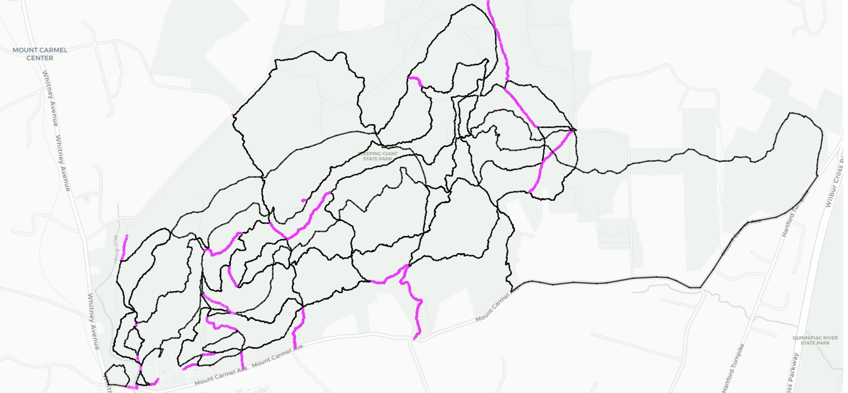
Edge walks per color:
black: 1
magenta: 2
fig, ax = plt.subplots(figsize=(1,10))

pos = {k: (grppviz.node[k]['lon'], grppviz.node[k]['lat']) for k in grppviz.nodes()}
e_width = [e[2]['linewidth'] for e in grppviz.edges(data=True)]
e_color = [e[2]['color_cnt'] for e in grppviz.edges(data=True)]
nx.draw_networkx_edges(grppviz, pos, width=e_width, edge_color=e_color, alpha=0.7)

mplleaflet.save_html(fig, 'maps/rpp_solution_edge_cnts.html', tiles='cartodb_positron')
Create geojson solution
Used for the D3 route animation at the beginning of the post (also here). More details here.
geojson = {'features':[], 'type': 'FeatureCollection'}
time = 0
path = list(reversed(circuit_rpp[0][3]['path']))

for e in circuit_rpp:
    if e[3]['path'][0] != path[-1]:
        path = list(reversed(e[3]['path']))
    else:
        path = e[3]['path']

    for n in path:
        time += 1
        doc = {'type': 'Feature',
              'properties': {
                  'latitude': g.node[n]['lat'],
                  'longitude': g.node[n]['lon'],
                  'time': time,
                  'id': e[3].get('id')
              },
              'geometry':{
                  'type': 'Point',
                  'coordinates': [g.node[n]['lon'], g.node[n]['lat']]
              }
          }
        geojson['features'].append(doc)
with open('circuit_rpp.geojson','w') as f:
    json.dump(geojson, f)